1. Introduction
This page serves as a 30,000-foot overview of the map-reduce programming paradigm and the key features that make it useful for solving certain types of computing workloads that simply cannot be treated using traditional parallel computing methods. It only covers the broad basics and is intended to provide you with the information you need to follow the subsequent pages I've written on:
- Writing Hadoop Applications in Python using Hadoop Streaming
- Parsing VCF files with Hadoop Streaming
- Parallel R using Hadoop
2. Comparing Map-Reduce to Traditional Parallelism
In order to appreciate what map-reduce brings to the table, I think it is most meaningful to contrast it to what I call traditional computing problems. I define "traditional" computing problems as those which use libraries like MPI, OpenMP, CUDA, or pthreads to produce results by utilizing multiple CPUs to perform some sort of numerical calculation concurrently. Problems that are well suited to being solved with these traditional methods typically share two common features:
- They are cpu-bound: the part of the problem that takes the most time is doing calculations involving floating point or integer arithmetic
- Input data is gigabyte-scale: the data that is necessary to describe the conditions of the calculation are typically less than a hundred gigabytes, and very often only a few hundred megabytes at most
Item #1 may seem trivial; after all, computers are meant to compute, so wouldn't all of the problems that need to be parallelized be fundamentally limited by how quickly the computer can do numerical calculations?
Traditionally, the answer to this question has been yes, but the technological landscape has been rapidly changing over the last decade. Sources of vast, unending data (e.g., social media, inexpensive genenome sequencing) have converged with inexpensive, high-capacity hard drives and the advanced filesystems to support them, and now data-intensive computing problems are emerging. In contrast to the aforementioned traditional computing problems, data-intensive problems demonstrate the following features:
- Input data is far beyond gigabyte-scale: datasets are commonly on the order of tens, hundreds, or thousands of terabytes
- They are I/O-bound: it takes longer for the computer to get data from its permanent location to the CPU than it takes for the CPU to operate on that data
2.1. Traditional Parallel Applications
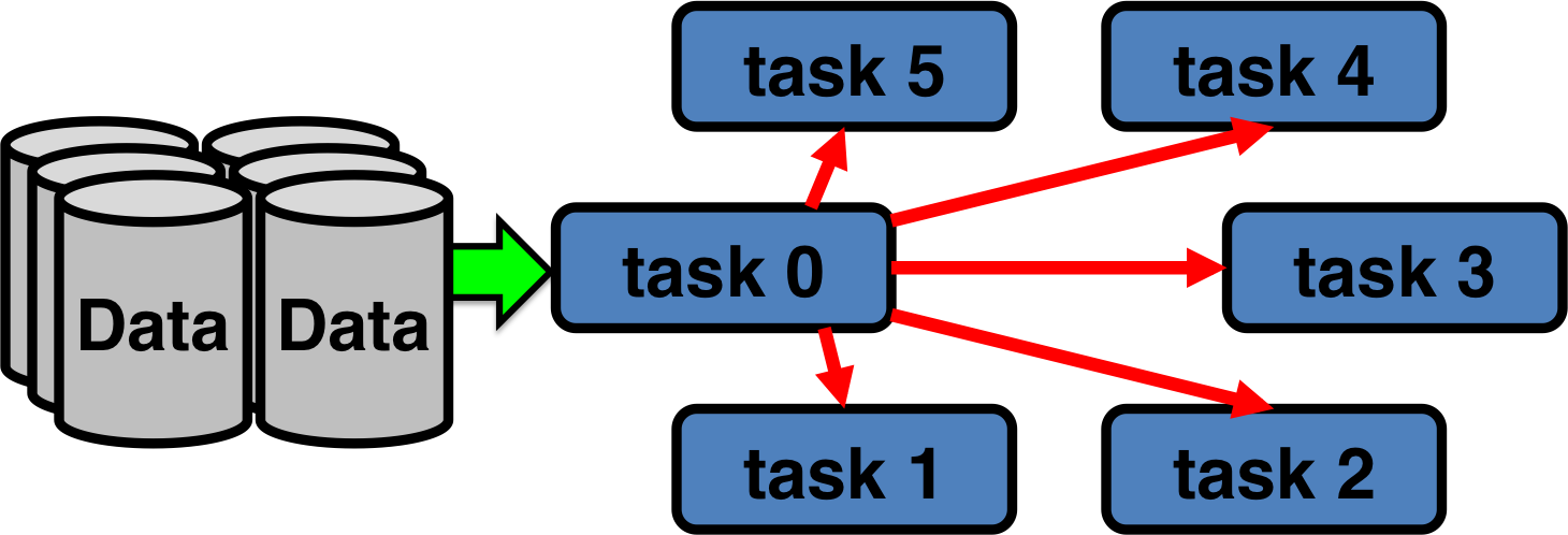
To illustrate these differences, the following schematic depicts how your typical traditionally parallel application works.

The input data is stored on some sort of remote storage device (a SAN, a file server serving files over NFS, a parallel Lustre or GPFS filesystem, etc; grey cylinders). The compute resources or elements (blue boxes) are abstract units that can represent MPI ranks, compute nodes, or threads on a shared-memory system.
Upon launching a traditionally parallel application,
- A master parallel worker (MPI rank, thread, etc) reads the input data from disk (green arrow).
- The master worker then divides up the input data into chunks and sends parts to each of the other workers (red arrows).
- All of the parallel workers compute their chunk of the input data
- All of the parallel workers communicate their results with each other, then continue the next iteration of the calculation
NOTE: In some cases multiple workers may use a parallel I/O API like MPI-IO to collectively read input data, but the filesystem on which the input data resides must be a high-performance filesystem that can sustain the required device- and network-read bandwidth.
The fundamental limit to scalability here is step #1--the process of reading the input data (green arrow) is performed serially. Even if you can use MPI-IO to perform the data ingestion in parallel, the data is separated from the compute resources (blue squares) by some pipe through which data can flow at some finite rate. While it is possible to increase the speed of this connection between your data and your compute resources by throwing more money at it (e.g., buying fast SSDs, faster storage networking, and/or more parallel storage servers), the cost of doing this does not scale linearly.
2.2. Data-intensive Applications
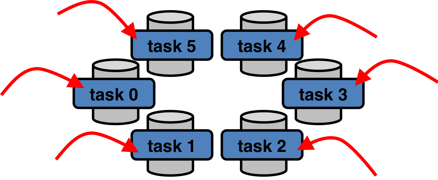
The map-reduce paradigm is a completely different way of solving a certain subset of parallelizable problems that gets around the bottleneck of ingesting input data from disk (that pesky green arrow). Whereas traditional parallelism brings the data to the compute, map-reduce does the opposite--it brings the compute to the data:

In map-reduce, the input data is not stored on a separate, high-capacity storage system. Rather, the data exists in little pieces and is permanently stored on the compute elements. This allows our parallel procedure to follow these steps:
- We don't have to move any data since it is pre-divided and already exists on nodes capable of acting as computing elements
- All of the parallel worker functions are sent to the nodes where their respective pieces of the input data already exist and do their calculations
- All of the parallel workers communicate their results with each other, move data if necessary, then continue the next step of the calculation
Thus, the only time data needs to be moved is when all of the parallel workers are communicating their results with each other in step #3. There is no more serial step where data is being loaded from a storage device before being distributed to the computing resources because the data already exists on the computing resources.
Of course, for the compute elements to be able to do their calculations on these chunks of input data, the calculations and data must be all completely independent from the input data on other compute elements. This is the principal constraint in map-reduce jobs: map-reduce is ideally suited for trivially parallel calculations on large quantities of data, but if each worker's calculations depend on data that resides on other nodes, you will begin to encounter rapidly diminishing returns.
3. Hadoop - A Map-Reduce Implementation
Now that we've established a description of the map-reduce paradigm and the concept of bringing compute to the data, we are equipped to look at Hadoop, an actual implementation of map-reduce.
3.1. The Magic of HDFS
The idea underpinning map-reduce--bringing compute to the data instead of the opposite--should sound like a very simple solution to the I/O bottleneck inherent in traditional parallelism. However, the devil is in the details, and implementing a framework where a single large file is transparently diced up and distributed across multiple physical computing elements (all while appearing to remain a single file to the user) is not trivial.
Hadoop, perhaps the most widely used map-reduce framework, accomplishes this feat using HDFS, the Hadoop Distributed File System. HDFS is fundamental to Hadoop because it provides the data chunking and distribution across compute elements necessary for map-reduce applications to be efficient. Since we're now talking about an actual map-reduce implementation and not an abstract concept, let's refer to the abstract compute elements now as compute nodes.
HDFS exists as a filesystem into which you can copy files to and from in a
manner not unlike any other filesystem. Many of the typical commands for
manipulating files (ls, mkdir, rm,
mv, cp, cat, tail, and
chmod, to name a few) behave as you might expect in any other
standard filesystem (e.g., Linux's ext4).
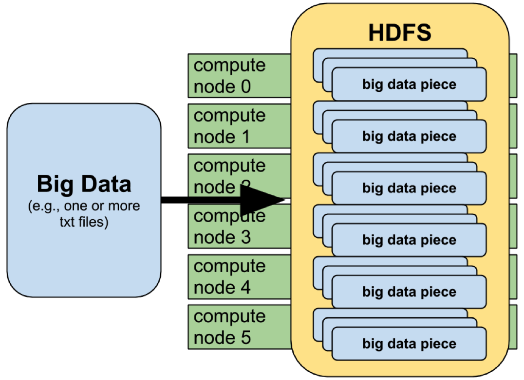
The magical part of HDFS is what is going on just underneath the surface. Although it appears to be a filesystem that contains files like any other, in reality those files are distributed across multiple physical compute nodes:

When you copy a file into HDFS as depicted above, that file is transparently sliced into 64 MB "chunks" and replicated three times for reliability. Each of these chunks are distributed to various compute nodes in the Hadoop cluster so that a given 64 MB chunk exists on three independent nodes. Although physically chunked up and distributed in triplicate, all of your interactions with the file on HDFS still make it appear as the same single file you copied into HDFS initially. Thus, HDFS handles all of the burden of slicing, distributing, and recombining your data for you.
The 64 MB chunk (block) size and the choice to replicate your data three times are only HDFS's default values. These decisions can be changed:
- the 64 MB block size can be modified by changing the
dfs.block.sizeproperty inhdfs-site.xml. It is common to increase this to 128 MB in production environments. - the replication factor can be modified by changing the
dfs.replicationproperty inhdfs-site.xml. It can also be changed on a per-file basis by specifying-D dfs.replication=1on your-putcommand line, or using the hadoop dfs -setrep -w 1 command.
3.2. Map-Reduce Jobs
HDFS is an interesting technology in that it provides data distribution, replication, and automatic recovery in a user-space filesystem that is relatively easy to configure and, conceptually, easy to understand. However, its true utility comes to light when map-reduce jobs are executed on data stored in HDFS.
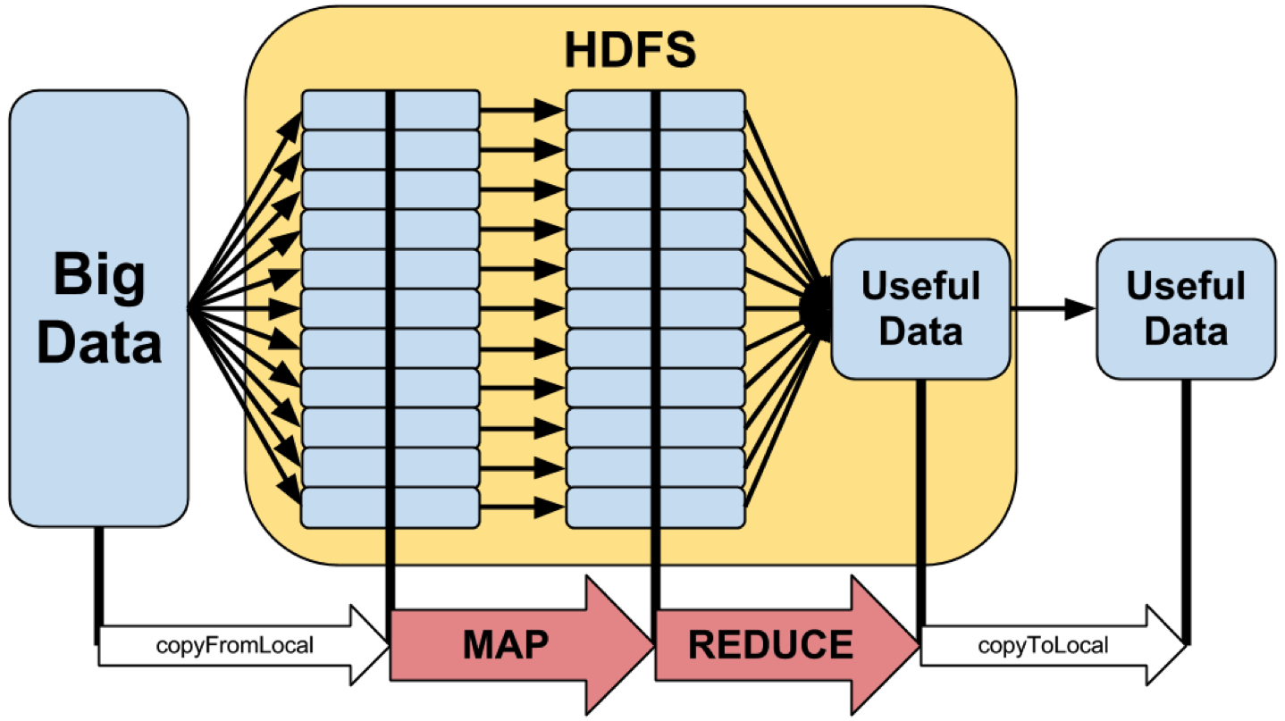
As the name implies, map-reduce jobs are principally comprised of two steps: the map step and the reduce step. The overall workflow generally looks something like this:

The left half of the diagram depicts the HDFS magic described in the previous section, where the hadoop dfs -copyFromLocal command is used to move a large data file into HDFS and it is automatically replicated and distributed across multiple physical compute nodes. While this step of moving data into HDFS is not strictly a part of a map-reduce job (i.e., your dataset may already have a permanent home on HDFS just like it would any other filesystem), a map-reduce job's input data must already exist on HDFS before the job can be started.
3.2.1. The Map Step
Once a map-reduce job is initiated, the map step
- Launches a number of parallel mappers across the compute nodes that contain chunks of your input data
- For each chunk, a mapper then "splits" the data into individual lines of
text on newline characters (
\n) - Each split (line of text that was terminated by
\n) is given to your mapper function - Your mapper function is expected to turn each line into zero or more key-value pairs and then "emit" these key-value pairs for the subsequent reduce step
That is, the map step's job is to transform your raw input data into a series of key-value pairs with the expectation that these parsed key-value pairs can be analyzed meaningfully by the reduce step. It's perfectly fine for duplicate keys to be emitted by mappers.
The decision to split your input data along newline characters is just the
default behavior, which assumes your input data is just an ascii text file.
You can change how input data is split before being passed to your mapper
function using alternate InputFormats.
3.2.2. The Reduce Step
Once all of the mappers have finished digesting the input data and have emitted all of their key-value pairs, those key-value pairs are sorted according to their keys and then passed on to the reducers. The reducers are given key-value pairs in such a way that all key-value pairs sharing the same key always go to the same reducer. The corollary is then that if one particular reducer has one specific key, it is guaranteed to have all other key-value pairs sharing that same key, and all those common keys will be in a continuous strip of key-value pairs that reducer received.
Your job's reducer function then does some sort of calculation based on all of the values that share a common key. For example, the reducer might calculate the sum of all values for each key (e.g., the word count example). The reducers then emit key-value pairs back to HDFS where each key is unique, and each of these unique keys' values are the result of the reducer function's calculation.
The process of sorting and distributing the mapper's output to the reducers
can be seen as a separate step often called the "shuffle". What really happens
is that as mappers emit key-value pairs, the keys are passed through the
Partitioner to determine which reducer they are sent to.
The default Partitioner is a function which hashes the key and
then takes the modulus of this hash and the number of reducers to determine
which reducer gets that key-value pair. Since the hash of a given key will
always be the same, all key-value pairs sharing the same key will get the same
output value from the Partitioner and therefore wind up on the
same reducer.
Once all key-value pairs are assigned to their reducers, the reducers all sort their keys so that a single loop over all of a reducer's keys will examine all the values of a single key before moving on to the next key. As you will see in the tutorial on writing mappers and reducers in Python that follows, this is an essential property of the Hadoop streaming interface.
This might sound a little complicated or abstract without an actual problem or sample code to examine; it is far easier to demonstrate what the reducer does by working through an example.
4. Summary
This conceptual overview of map-reduce and Hadoop is admittedly dry without a meaningful example to accompany it, so here are the key points you should take away:
- map-reduce brings compute to the data in contrast to traditional parallelism, which brings data to the compute resources
- Hadoop accomplishes this by storing data in a replicated and distributed fashion on HDFS
- HDFS stores files in chunks which are physically stored on multiple compute nodes
- HDFS still presents data to users and applications as single continuous files despite the above fact
- map-reduce is ideal for operating on very large, flat (unstructured) datasets and perform trivially parallel operations on them
- Hadoop jobs go through a map stage and a reduce stage where
- the mapper transforms the raw input data into key-value pairs where multiple values for the same key may occur
- the reducer transforms all of the key-value pairs sharing a common key into a single key with a single value
If you have any interest remaining after having read this, I strongly recommend looking through my tutorial on Writing Hadoop Applications in Python with Hadoop Streaming. That tutorial covers much of the same material, but in the context of an actual problem (counting the number of times each word appears in a text) with actual code written in Python.